데이터 사이언스와 디자인

디자인과 아키텍쳐의 중요성

이광춘, 한국 R 사용자회

2022-10-11

github.com/bit2r/quarto

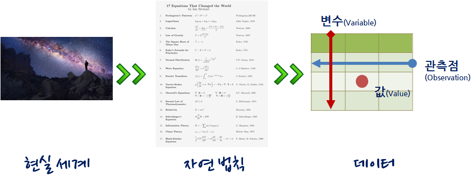
데이터 사이언스

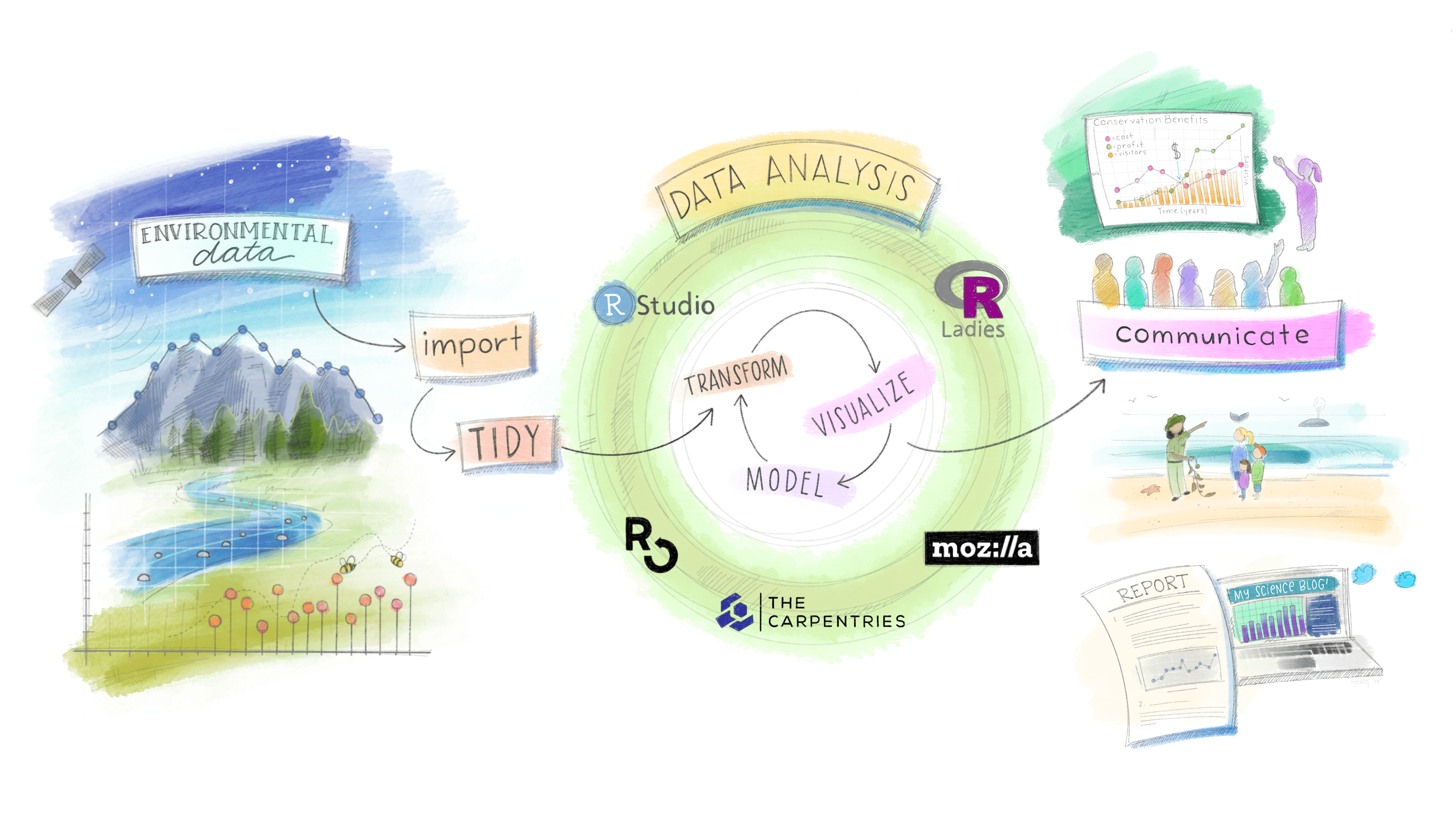
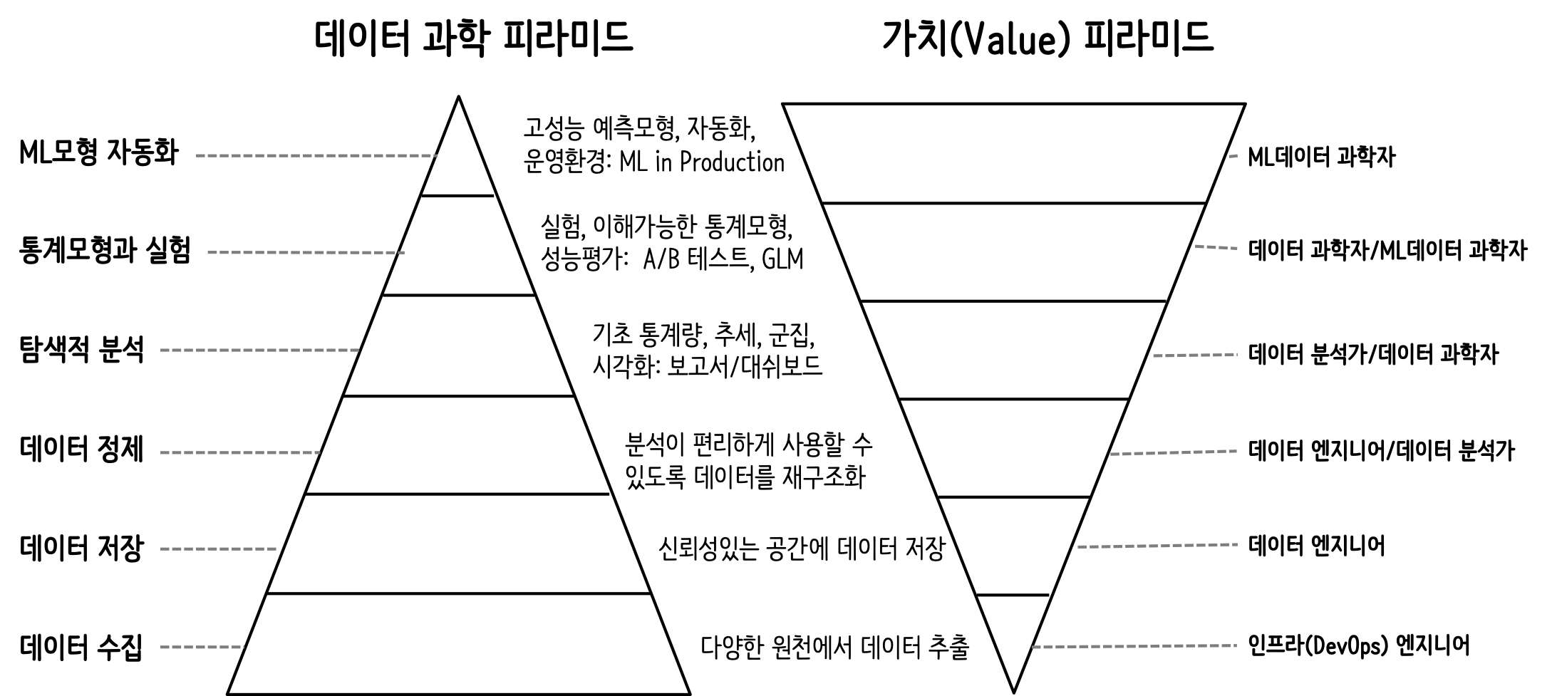
데이터 과학 욕구단계설

매슬로 욕구단계설
가치 피라미드

데이터 과학 문제

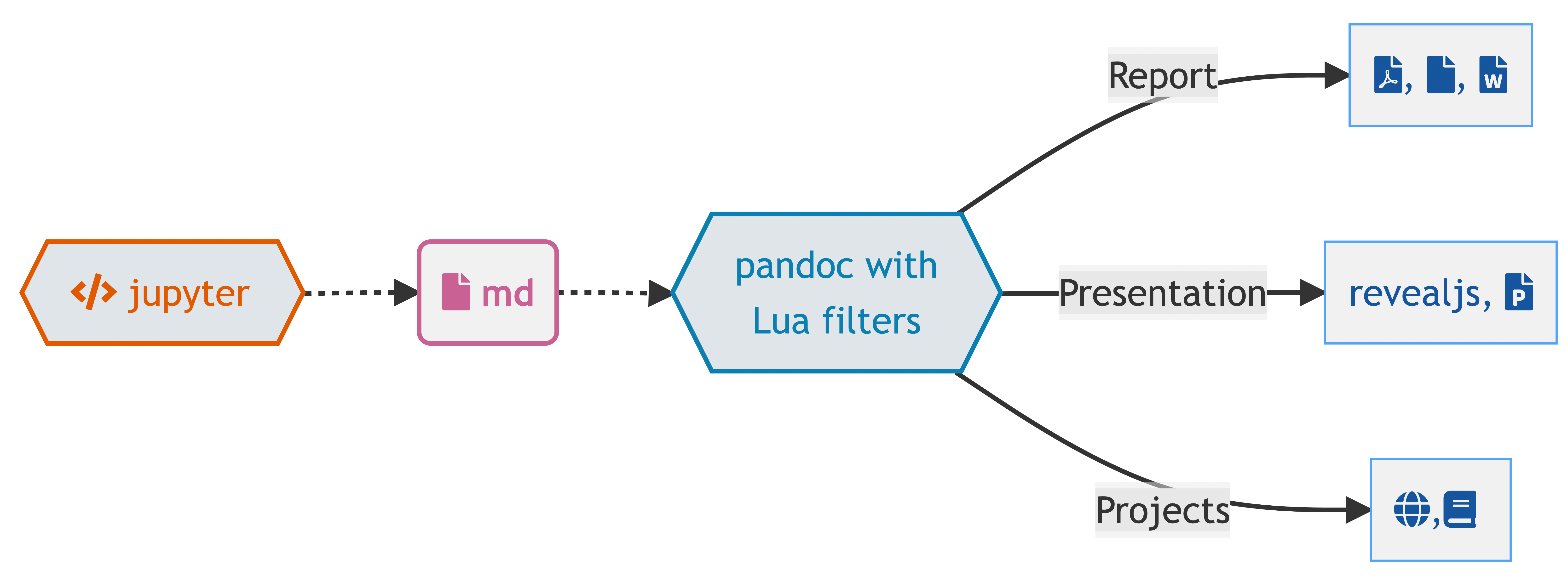
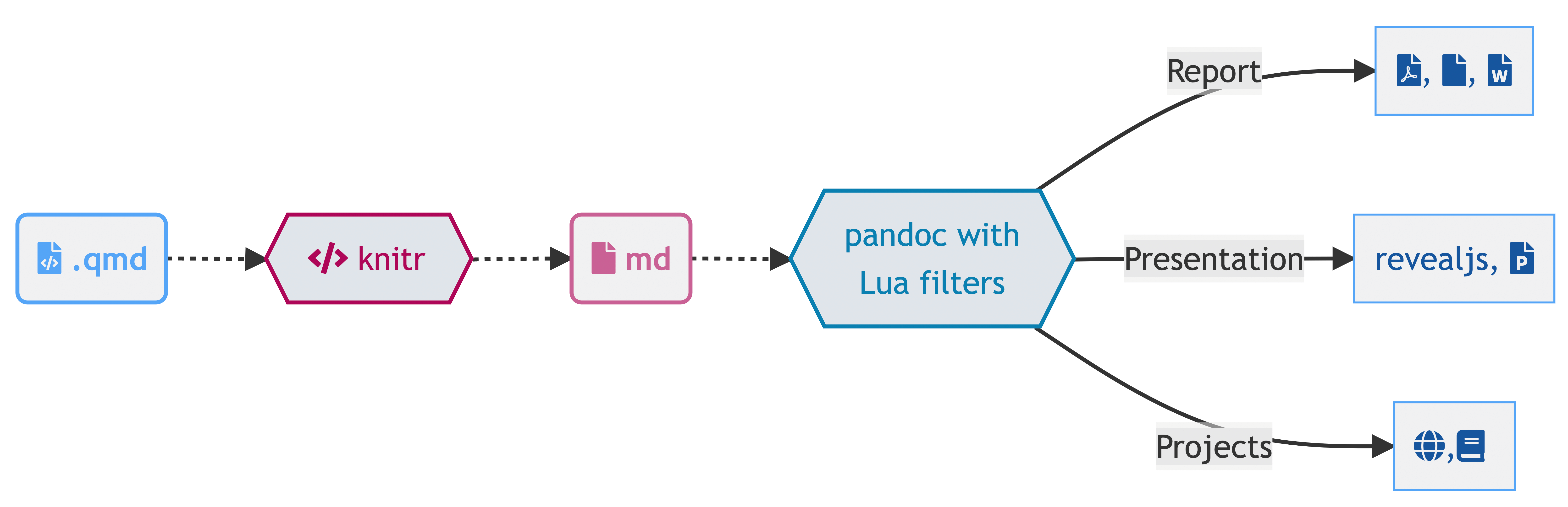
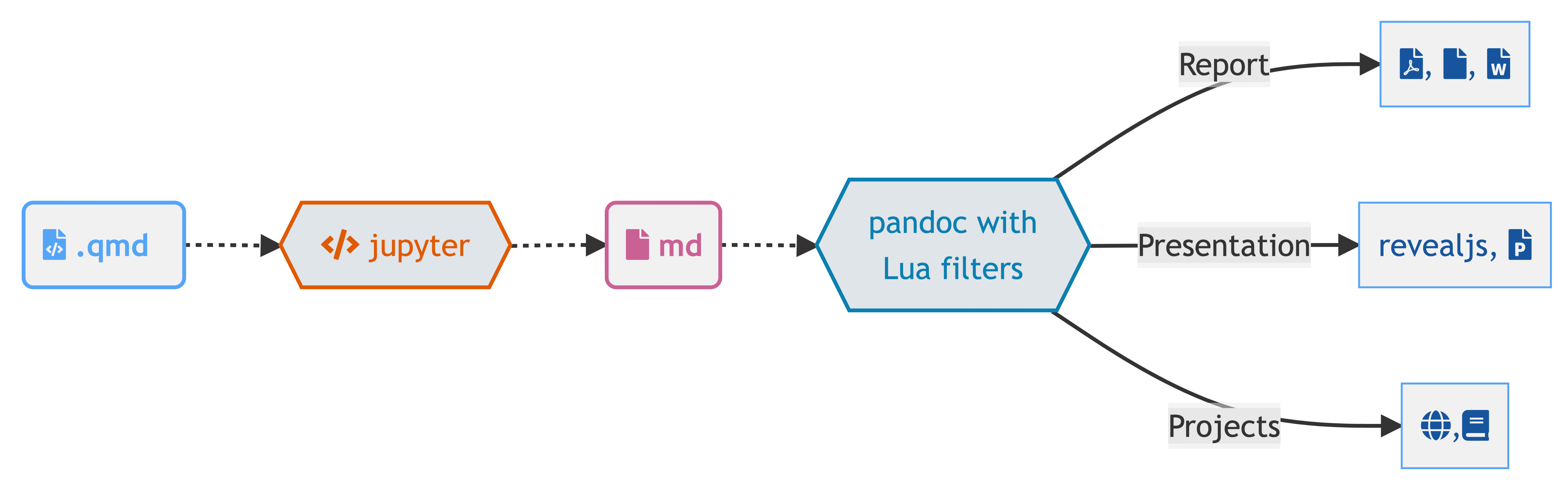
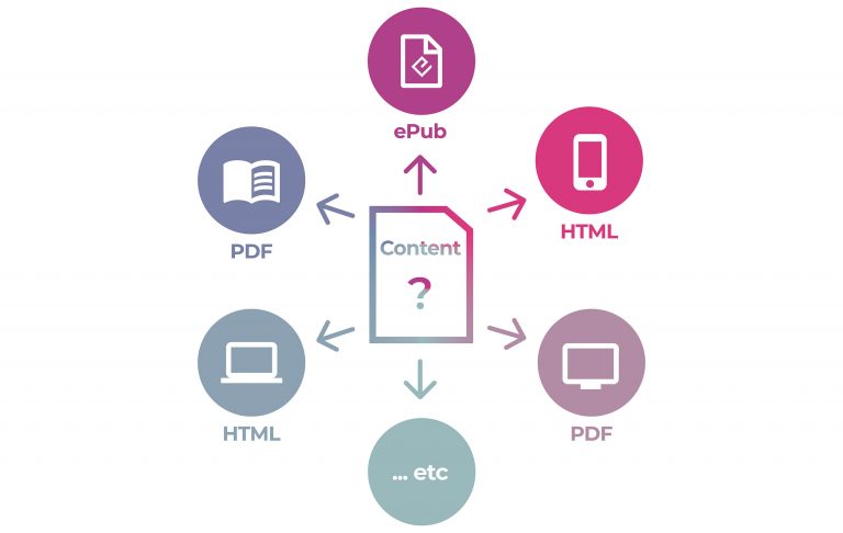
데이터 사이언스 - 출판

문제점
개념
Single Sourcing Multi-Use

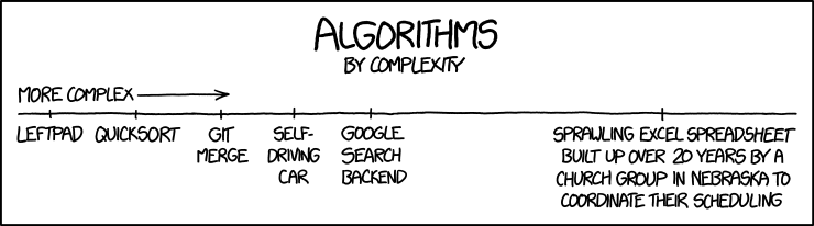
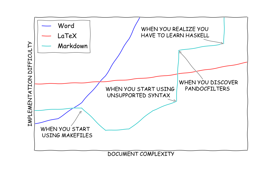
복잡성

엑셀 ¹
아래한글 ²

시각화 - 그래프 문법 ¹

R 코드

library(tidyverse)
bill_df <- data.frame(
  sex = factor(c("여성","여성","남성","남성")),
  time = factor(c("점심","저녁","점심","저녁"), levels=c("점심","저녁")),
  total_bill = c(13.53, 16.81, 16.24, 17.42)
)

실행결과

bill_df

   sex time total_bill
1 여성 점심      13.53
2 여성 저녁      16.81
3 남성 점심      16.24
4 남성 저녁      17.42

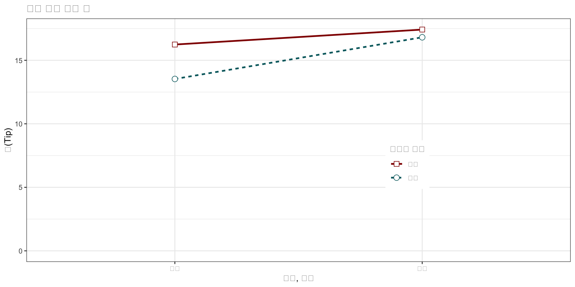
R 코드

bill_df %>% 
  ggplot(aes(x=time, y=total_bill, group=sex, shape=sex, colour=sex)) +
    geom_line(aes(linetype=sex), size=1) +    
    geom_point(size=3, fill="white") +        
    expand_limits(y=0) +                      
    scale_colour_hue(name="결재자 성별", l=30) +
    scale_shape_manual(name="결재자 성별", values=c(22,21)) +
    scale_linetype_discrete(name="결재자 성별") +
    xlab("점심, 석식") + ylab("팁(Tip)") +
    ggtitle("식사 결재 평균 팁") +    
    theme_bw() +
    theme(legend.position=c(.7, .4))

실행결과

R 코드

bill_mat <- matrix( bill_df$total_bill,
                   nrow = 2,
                   byrow=TRUE,
                   dimnames = list(c("여성", "남성"), c("점심", "저녁"))
                   )

mf_col <- c("#3CC3BD", "#FD8210")
barplot(bill_mat, beside = TRUE, border=NA, col=mf_col)
legend("topleft", row.names(bill_mat), pch=15, col=mf_col)


par(cex=1.2, cex.axis=1.1)
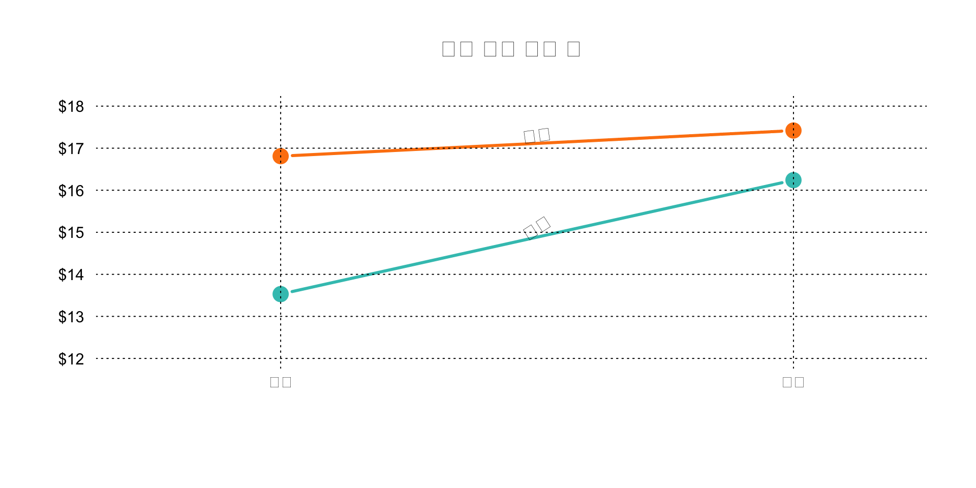
matplot(bill_mat, type="b", lty=1, pch=19, col=mf_col,
    cex=1.5, lwd=3, las=1, bty="n", xaxt="n",
    xlim=c(0.7, 2.2), ylim=c(12,18), ylab="",
    main="식사 결재 평균 팁", yaxt="n")
axis(2, at=axTicks(2), labels=sprintf("$%s", axTicks(2)),
    las=1, cex.axis=0.8, col=NA, line = -0.5)
grid(NA, NULL, lty=3, lwd=1, col="#000000")
abline(v=c(1,2), lty=3, lwd=1, col="#000000")
mtext("점심", side=1, at=1)
mtext("저녁", side=1, at=2)
text(1.5, 17.3, "남성", srt=8, font=3)
text(1.5, 15.1, "여성", srt=33, font=3)

실행결과

디자인 - 코드

데이터 가공
dplyr R
Base R
SQL
파이썬

날짜와 시간별로 총 빈도수와 출발연착 평균 시간을 구한다. 단, 총빈도수가 10 회 미만인 것은 제외하고 출발연착 시간의 결측값을 제거하고 계산한다.

flights 데이터프레임에서
출발 연착시간(dep_delay) 칼럼에서 결측값이 없는 (!is.na()) 행을 필터링 하고
날짜별(date), 시간별(hour) 그룹을 묶어
평균 출발 연착시간을 계산하고 총빈도수 총계를 내고
총빈도수가 10회 이상인 날짜와 시간을 찾아내시오

hourly_delay <- flights %>%  
  filter(!is.na(dep_delay)) %>% 
  group_by(date, hour) %>% 
  summarise(delay = mean(dep_delay), n = n()) %>%  
  filter(n > 10)

hourly_delay <- filter(   
    summarise(   
        group_by(   
             filter(   
                 flights,    
                 !is.na(dep_delay)   
             ),    
             date, hour   
        ),    
    delay = mean(dep_delay),    
         n = n()   
    ),    
    n > 10   
)

SELECT "date", "hour", "delay", "n"
FROM (
    SELECT "date", "hour",
        AVG("dep_delay") AS "delay",
        COUNT() AS "n"
    FROM "flights"
    WHERE NOT("dep_delay" IS NULL)
    GROUP BY "date", "hour"
) AS "_W1"
WHERE "n" > 10.0

flights[['date','hour','dep_delay']]
...

WHO 결핵 원데이터
WHO 에서 년도별, 국가별, 연령별, 성별, 진단방법별 결핵 발병사례 조사 통계 데이터
진단방법
- rel stands for cases of relapse
- ep stands for cases of extrapulmonary TB
- sn stands for cases of pulmonary TB that could not be diagnosed by a pulmonary smear (smear negative)
- sp stands for cases of pulmonary TB that could be diagnosed by a pulmonary smear (smear positive)
연령
- 014 = 0 – 14 years old
- 1524 = 15 – 24 years old
- 2534 = 25 – 34 years old
- 3544 = 35 – 44 years old
- 4554 = 45 – 54 years old
- 5564 = 55 – 64 years old
- 65 = 65 or older
성별
- males (m)
- females (f)

library(tidyverse)
tidyr::who

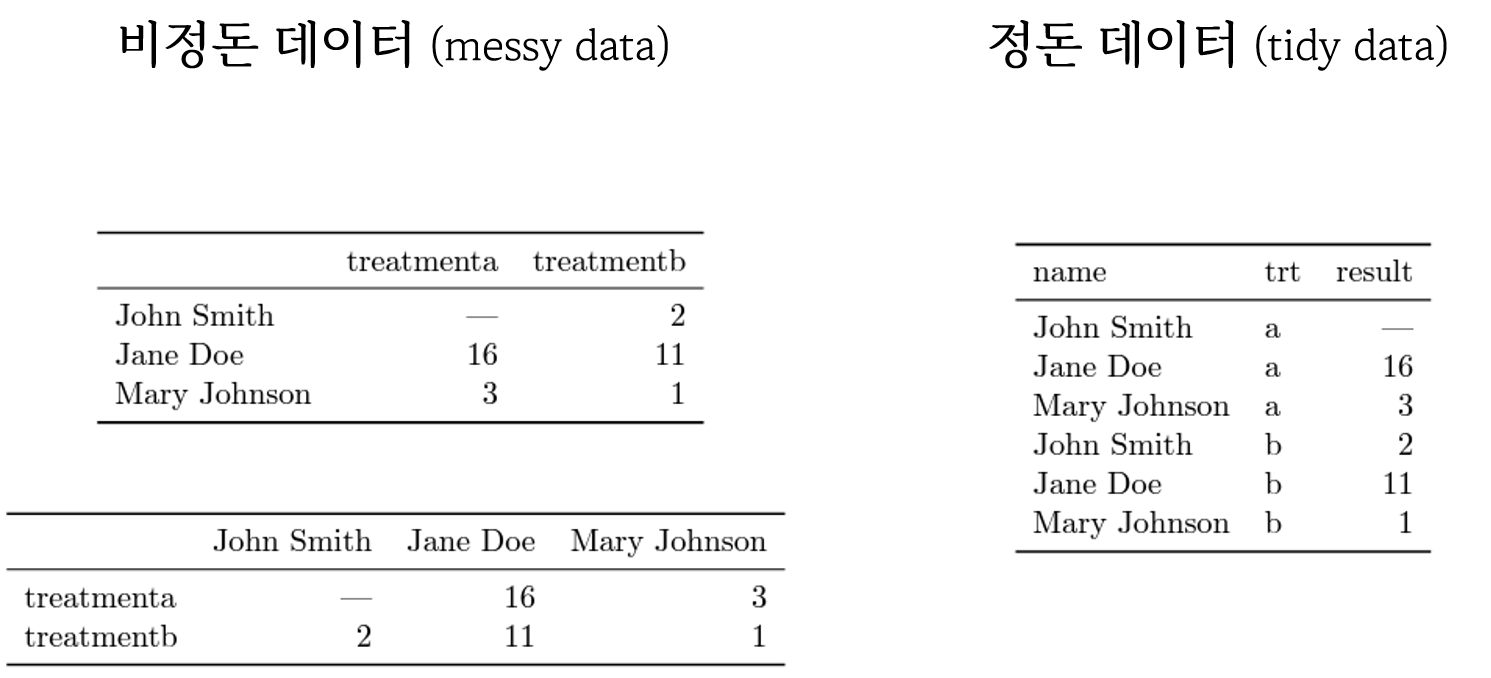
# A tibble: 7,240 × 60
   country     iso2  iso3   year new_s…¹ new_s…² new_s…³ new_s…⁴ new_s…⁵ new_s…⁶
   <chr>       <chr> <chr> <int>   <int>   <int>   <int>   <int>   <int>   <int>
 1 Afghanistan AF    AFG    1980      NA      NA      NA      NA      NA      NA
 2 Afghanistan AF    AFG    1981      NA      NA      NA      NA      NA      NA
 3 Afghanistan AF    AFG    1982      NA      NA      NA      NA      NA      NA
 4 Afghanistan AF    AFG    1983      NA      NA      NA      NA      NA      NA
 5 Afghanistan AF    AFG    1984      NA      NA      NA      NA      NA      NA
 6 Afghanistan AF    AFG    1985      NA      NA      NA      NA      NA      NA
 7 Afghanistan AF    AFG    1986      NA      NA      NA      NA      NA      NA
 8 Afghanistan AF    AFG    1987      NA      NA      NA      NA      NA      NA
 9 Afghanistan AF    AFG    1988      NA      NA      NA      NA      NA      NA
10 Afghanistan AF    AFG    1989      NA      NA      NA      NA      NA      NA
# … with 7,230 more rows, 50 more variables: new_sp_m65 <int>,
#   new_sp_f014 <int>, new_sp_f1524 <int>, new_sp_f2534 <int>,
#   new_sp_f3544 <int>, new_sp_f4554 <int>, new_sp_f5564 <int>,
#   new_sp_f65 <int>, new_sn_m014 <int>, new_sn_m1524 <int>,
#   new_sn_m2534 <int>, new_sn_m3544 <int>, new_sn_m4554 <int>,
#   new_sn_m5564 <int>, new_sn_m65 <int>, new_sn_f014 <int>,
#   new_sn_f1524 <int>, new_sn_f2534 <int>, new_sn_f3544 <int>, …

who %>%
  pivot_longer(
    cols = new_sp_m014:newrel_f65, 
    names_to = "key", 
    values_to = "cases", 
    values_drop_na = TRUE
  ) %>% 
  mutate(
    key = stringr::str_replace(key, "newrel", "new_rel")
  ) %>%
  separate(key, c("new", "var", "sexage")) %>% 
  select(-new, -iso2, -iso3) %>% 
  separate(sexage, c("sex", "age"), sep = 1)

# A tibble: 76,046 × 6
   country      year var   sex   age   cases
   <chr>       <int> <chr> <chr> <chr> <int>
 1 Afghanistan  1997 sp    m     014       0
 2 Afghanistan  1997 sp    m     1524     10
 3 Afghanistan  1997 sp    m     2534      6
 4 Afghanistan  1997 sp    m     3544      3
 5 Afghanistan  1997 sp    m     4554      5
 6 Afghanistan  1997 sp    m     5564      2
 7 Afghanistan  1997 sp    m     65        0
 8 Afghanistan  1997 sp    f     014       5
 9 Afghanistan  1997 sp    f     1524     38
10 Afghanistan  1997 sp    f     2534     36
# … with 76,036 more rows